16. Carbon Modelling Practical : Answers to exercises
Binder ![]()
Answers ![]()
[1]:
import numpy as np
import matplotlib.pyplot as plt
from geog0133.photJules import photosynthesis
from geog0133.photter import plotme,day_plot,gpp_plot
from geog0133.solar import radiation
from geog0133.pp import daily_PP,annual_npp
from geog0133.cru import getCRU,splurge
from matplotlib import animation
from datetime import datetime, timedelta
# import codes we need into the notebook


def do_photosynthesis(ipar=200.,Tc=None,co2_ppmv=390,n=100,
          pft_type='C3 grass',plotter=None,x=None):
    '''
    A function to run the photosynthesis model.

    Function allows the user to change
    a number of important photosynthesis parameters:

    incoming PAR radiation, canopy temperature, CO2 concentration,
    C3/C4 pathway and the PFT type. The first three
    parameters can be provided as arrays.

    The function will produce a plot of the variation
    of photosynthesis as it sweeps over the parameter range.
    '''
    from geog0133.photJules import photosynthesis
    photo = photosynthesis()
    photo.data = np.zeros(n)

    # set plant type to C3
    if pft_type == 'C4 grass':
        photo.C3 = np.zeros([n]).astype(bool)
    else:
        photo.C3 = np.ones([n]).astype(bool)

    photo.Lcarbon = np.ones([n]) * 1
    photo.Rcarbon = np.ones([n]) * 1
    photo.Scarbon = np.ones([n]) * 1

    # set pft type
    # options are:
    # 'C3 grass', 'C4 grass', 'Needleleaf tree', 'Shrub'
    # 'Broadleaf tree'
    # Note that if C4 used, you must set the array
    # self.C3 to False

    photo.pft = np.array([pft_type]*n)

    # set up Ipar, incident PAR in (mol m-2 s-1)
    photo.Ipar = np.ones_like(photo.data) * ipar * 1e-6

    # set co2 (ppmv)
    photo.co2_ppmv = co2_ppmv*np.ones_like(photo.data)

    # set up a temperature range (C)
    try:
        if Tc is None:
            photo.Tc = Tc or np.arange(n)/(1.*n) * 100. - 30.
        else:
            photo.Tc = Tc
    except:
        photo.Tc = Tc

    # initialise
    photo.initialise()
    # reset defaults
    photo.defaults()

    # calculate leaf and canopy photosynthesis
    photo.photosynthesis()
    try:
        if x == None:
            x = photo.Tc
    except:
        pass
    plotter = plotme(x,photo,plotter)

    return photo,plotter
16.1. Exercise
Light-limiting assimilation
We repeat Table 2 from Clark et al., 2011 for convenience:
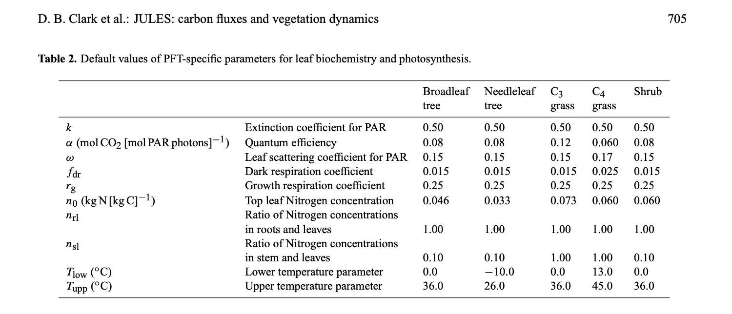
From the data in this table and your understanding of the controls on photosynthesis in the model, answer the following questions and confirm your answer by running the model.
which PFT has the highest values of
We, and why?How does this change with increasing
ipar?When ipar is the limiting factor, how does assimilation change when ipar increases by a factor of k?
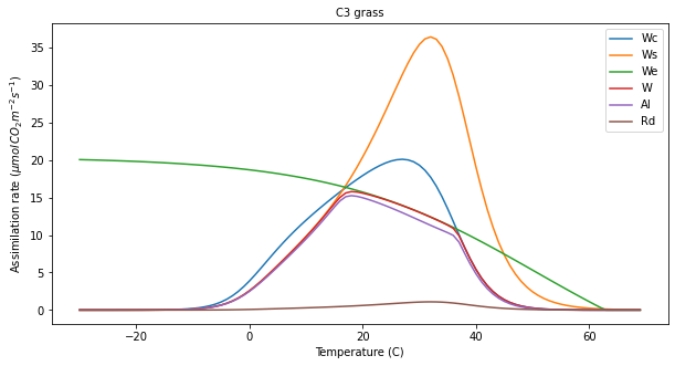
For C3 grasses, what are the limiting factors over the temperatures modelled for ipar=200?
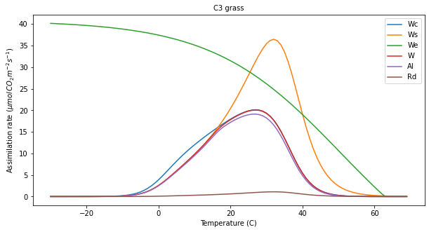
For C3 grasses, what are the limiting factors over the temperatures modelled for ipar=400?
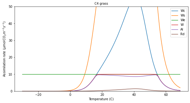
For C4 grasses, what are the limiting factors over the temperatures modelled?
[2]:
#### ANSWER

msg = f'''
which PFT has the highest values of We, and why?

From the notes, product of the quantum efficiency alpha,
the PAR absorption rate (ipar) and the leaf absorptance
(1 - omega, where omega is the leaf single scattering albedo).

So, for given ipar, it is controlled by the product of
alpha and (1 - omega).

The C3 plants have the same value of omega here (0.15)
so 1 - omega = 0.85. For C4, this is 0.83.

C3 grasses have the highest value of alpha (0.12).

So,
For C3 max, we have alpha * (1 - omega) = 0.85 * 0.12 = {0.85 * 0.12}
For C4    , we have alpha * (1 - omega) = 0.83 * 0.06 = {0.83 * 0.06}

so, C3 grasses should have the highest We.

The other C3 plants should have the same We curves.

We can demonstrate this:

Maximum We for each PFT for default CO2 and ipar
'''


print(msg)

# list of all pfts
pfts = ['C3 grass','C4 grass',\
            'Broadleaf tree','Needleleaf tree','Shrub']
# store the data for each PFT
output = {}
# loop over pfts
for pft in pfts:
    output[pft],plotter = do_photosynthesis(ipar=200,pft_type=pft)
    print(pft,output[pft].We.max() * 1e6,'umolCO2m-2s-1')
which PFT has the highest values of We, and why?

From the notes, product of the quantum efficiency alpha,
the PAR absorption rate (ipar) and the leaf absorptance
(1 - omega, where omega is the leaf single scattering albedo).

So, for given ipar, it is controlled by the product of
alpha and (1 - omega).

The C3 plants have the same value of omega here (0.15)
so 1 - omega = 0.85. For C4, this is 0.83.

C3 grasses have the highest value of alpha (0.12).

So,
For C3 max, we have alpha * (1 - omega) = 0.85 * 0.12 = 0.102
For C4    , we have alpha * (1 - omega) = 0.83 * 0.06 = 0.0498

so, C3 grasses should have the highest We.

The other C3 plants should have the same We curves.

We can demonstrate this:

Maximum We for each PFT for default CO2 and ipar

C3 grass 20.07264113525945 umolCO2m-2s-1
C4 grass 9.959999999999997 umolCO2m-2s-1
Broadleaf tree 13.381760756839634 umolCO2m-2s-1
Needleleaf tree 13.381760756839634 umolCO2m-2s-1
Shrub 13.381760756839634 umolCO2m-2s-1
[3]:
#### ANSWER
msg = '''
How does this change with increasing ipar?

It scales with ipar, so increasing ipar increases We

'''
print(msg)
output = {}
pfts = ['C3 grass','C4 grass']
for pft in pfts:
    output[pft],plotter = do_photosynthesis(pft_type=pft,ipar=200.)
    print(pft,'ipar=200',output[pft].We.max() * 1e6,'umolCO2m-2s-1')
    output[pft],plotter = do_photosynthesis(pft_type=pft,ipar=400.)
    print(pft,'ipar=400',output[pft].We.max() * 1e6,'umolCO2m-2s-1')
How does this change with increasing ipar?

It scales with ipar, so increasing ipar increases We


C3 grass ipar=200 20.07264113525945 umolCO2m-2s-1
C3 grass ipar=400 40.1452822705189 umolCO2m-2s-1
C4 grass ipar=200 9.959999999999997 umolCO2m-2s-1
C4 grass ipar=400 19.919999999999995 umolCO2m-2s-1
[4]:
#### ANSWER

msg = '''
When ipar is the limiting factor, how does assimilation change
when ipar increases by a factor of k?

This is almost the same question as above:

When ipar is the limiting factor (for all cases) it scales
directly with the value of ipar -- so increasing ipar by a factor of
k will increase assimilation by that same factor.
'''
print(msg)
When ipar is the limiting factor, how does assimilation change
when ipar increases by a factor of k?

This is almost the same question as above:

When ipar is the limiting factor (for all cases) it scales
directly with the value of ipar -- so increasing ipar by a factor of
k will increase assimilation by that same factor.
[5]:
### ANSWER
msg = '''
For C3 grasses, what are the limiting factors over the temperatures modelled for ipar=200?
'''

# list of all pfts
pfts = ['C3 grass']

plotter = {
    'n_subplots' : len(pfts),       # number of sub-plots
    'name'       : 'default',  # plot name
    'ymax'        : None      # max value for y set
}

# store the data for each PFT
output = {}
# loop over pfts
for pft in pfts:
    output[pft],plotter = do_photosynthesis(ipar=200,pft_type=pft,plotter=plotter)

msg = '''
With ipar=200 and co2_ppmv=390, we have the same graph we saw earlier.
The limiting factors are Ws up to around 17 C
(close to We value), then We to around 36 C
then Wc. At moderate temperatures then, and low ipar,
light is the main limiting factor. At lower temperatures
it is transport-limited (almost the same as carboxylation)
and at higher tempertures it is limited by carboxylation.
'''
print(msg)
>>> Saved result in photter_default.png

With ipar=200 and co2_ppmv=390, we have the same graph we saw earlier.
The limiting factors are Ws up to around 17 C
(close to We value), then We to around 36 C
then Wc. At moderate temperatures then, and low ipar,
light is the main limiting factor. At lower temperatures
it is transport-limited (almost the same as carboxylation)
and at higher tempertures it is limited by carboxylation.
[6]:
### ANSWER
msg = '''
For C3 grasses, what are the limiting factors over the temperatures modelled for ipar=400?
'''

# list of all pfts
pfts = ['C3 grass']

plotter = {
    'n_subplots' : len(pfts),       # number of sub-plots
    'name'       : 'default',  # plot name
    'ymax'        : None      # max value for y set
}

# store the data for each PFT
output = {}
# loop over pfts
for pft in pfts:
    output[pft],plotter = do_photosynthesis(ipar=400,pft_type=pft,plotter=plotter)

msg = '''
With ipar=400 and co2_ppmv=390, we have removed the
light limitation. The main shape follows closely
that of Wc, though up to around 17 C it is
actually Ws that is limiting here.
'''
print(msg)
>>> Saved result in photter_default.png

With ipar=400 and co2_ppmv=390, we have removed the
light limitation. The main shape follows closely
that of Wc, though up to around 17 C it is
actually Ws that is limiting here.
[7]:
### ANSWER
msg = '''
For C4 grasses, what are the limiting factors over the temperatures modelled?
'''
# list of all pfts
pfts = ['C4 grass']
# set ymax here to be able to see the plots
plotter = {
'n_subplots' : len(pfts), # number of sub-plots
'name' : 'default', # plot name
'ymax' : 50 # max value for y set
}
# store the data for each PFT
output = {}
# loop over pfts
for pft in pfts:
output[pft],plotter = do_photosynthesis(ipar=200,pft_type=pft,plotter=plotter)
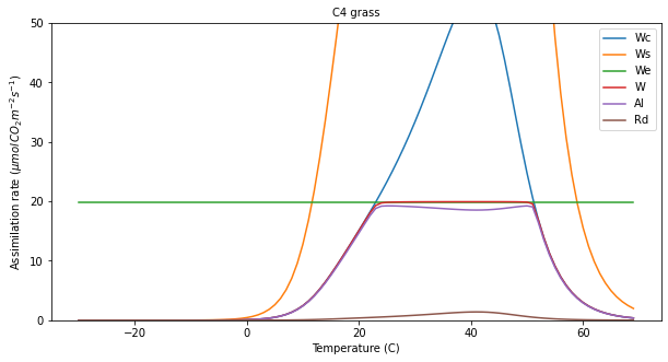
msg = '''
With ipar=200 and co2_ppmv=390, we have the same graph we saw earlier.
The limiting factors are Wc up to around 17 C and after 36 C.
For moderate temperatures, it is light limited. The light-limited rate
defines the maximum assimilation rate.
'''
print(msg)
>>> Saved result in photter_default.png

With ipar=200 and co2_ppmv=390, we have the same graph we saw earlier.
The limiting factors are Wc up to around 17 C and after 36 C.
For moderate temperatures, it is light limited. The light-limited rate
defines the maximum assimilation rate.
[8]:
#### ANSWER

# list of all pfts
pfts = ['C4 grass']

# store the data for each PFT
output = {}
# set ymax here to be able to see the plots
plotter = {
    'n_subplots' : len(pfts),       # number of sub-plots
    'name'       : 'default',  # plot name
    'ymax'        : 50      # max value for y set
}

# loop over pfts
for pft in pfts:
    output[pft],plotter = do_photosynthesis(ipar=400,pft_type=pft,plotter=plotter)

msg = '''
As we increase ipar, we reduce the temperature range at which
light limitation kicks in, and increase the maximum rate
proportionately by the proportionate increase in ipar.
'''
print(msg)
>>> Saved result in photter_default.png

As we increase ipar, we reduce the temperature range at which
light limitation kicks in, and increase the maximum rate
proportionately by the proportionate increase in ipar.
16.2. Exercise
Explain the factors limiting Carbon assimilation for several PFTs, latitudes and time of year
You should relate your answer to the plots on assimilation as a function of temperature we examined earlier.
[9]:
# ANSWER : C3 grass

latitude = 23.5
longitude = 30

pft = "C3 grass"
year = 2019
doys = [80,172,264,355]

params = []
for i,doy in enumerate(doys):
    jd,ipar,Tc = radiation(latitude,longitude,doy,year=year)
    p = do_photosynthesis(n=len(ipar), pft_type=pft,Tc=Tc, \
                          ipar=ipar,co2_ppmv=390,\
                          x=ipar,plotter=None)[0]
    params.append((jd,ipar,Tc,p,doy))

# plotting code
day_plot(params,title=f'{pft}: lat {latitude} lon {longitude}')
[10]:
# ANSWER : C4 grass

latitude = 23.5
longitude = 30

pft = "C4 grass"

year = 2019
doys = [80,172,264,355]

params = []
for i,doy in enumerate(doys):
    jd,ipar,Tc = radiation(latitude,longitude,doy,year=year)
    p = do_photosynthesis(n=len(ipar), pft_type=pft,Tc=Tc, \
                          ipar=ipar,co2_ppmv=390,\
                          x=ipar,plotter=None)[0]
    params.append((jd,ipar,Tc,p,doy))

# plotting code
day_plot(params,title=f'{pft}: lat {latitude} lon {longitude}')
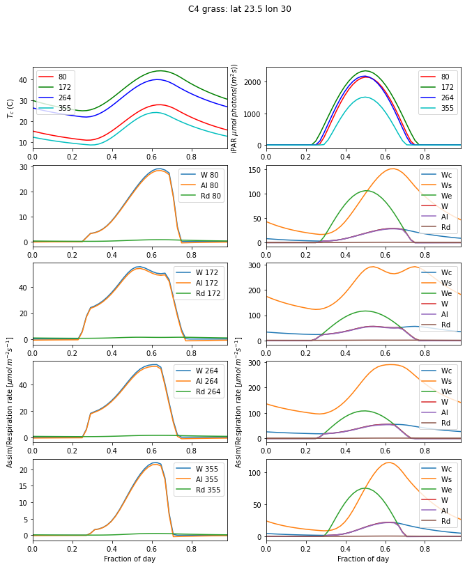
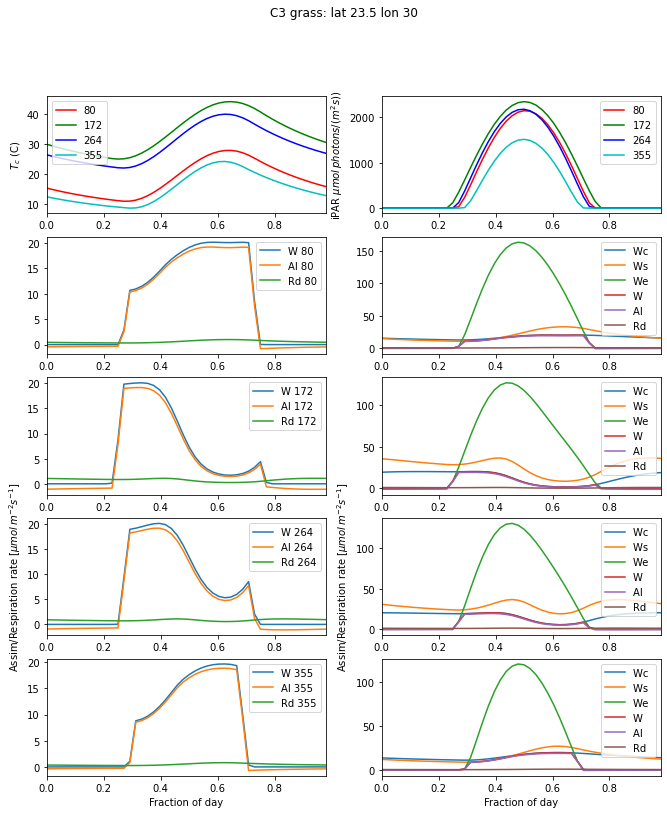
[11]:
msg = '''
Explain the factors limiting Carbon assimilation for several PFTs, latitudes and time of year
You should relate your answer to the plots on assimilation as a function of temperature we examined earlier.

We show an example of C3 and C4 grass at the tropic of Cancer

First, we notice that the assimilation rate is significantly higher
for the C4 grass than for a C3 grass.

Light limitation kicks in with the daytime as we have previosly seen.

The temperature ranges for C3 and C4 grasses are : 0-36 C and 13-45 C
respectively. At days 172 and 264, we see the temperature is sometimes
above the upper limit for C3 grass, and both Ws and Wc are very low
during this period, and the assimilation rate is close to zero all afternoon.
This is not the case for the more temperature-tolerant C4 grasses. For days
80 and 355, the temperature is more comfortable for both types of grass
and assimilation broadly follows the temperature increase over the day.
'''
print(msg)
Explain the factors limiting Carbon assimilation for several PFTs, latitudes and time of year
You should relate your answer to the plots on assimilation as a function of temperature we examined earlier.

We show an example of C3 and C4 grass at the tropic of Cancer

First, we notice that the assimilation rate is significantly higher
for the C4 grass than for a C3 grass.

Light limitation kicks in with the daytime as we have previosly seen.

The temperature ranges for C3 and C4 grasses are : 0-36 C and 13-45 C
respectively. At days 172 and 264, we see the temperature is sometimes
above the upper limit for C3 grass, and both Ws and Wc are very low
during this period, and the assimilation rate is close to zero all afternoon.
This is not the case for the more temperature-tolerant C4 grasses. For days
80 and 355, the temperature is more comfortable for both types of grass
and assimilation broadly follows the temperature increase over the day.